Join Metrics Queries

You can join metrics queries to combine, compare, and perform operations on the results of multiple queries.

By using the along statement in joins, you can control what results are joined, based on the value of one or more result fields.

Syntax

<expression> [along <field>[, <field>, …]]

Why use along?​

This section explains the benefit of using along when you join metrics queries.

In the Metrics Explorer you can run up to six separate queries and display and compare the query results on the same chart. The queries are labeled from #A to #F.

You can combine (join) the results of multiple queries, or use values from one query to filter values from another.

Here’s an example of a simple join that sums two metrics:

#C: #A + #B

This join works fine, if each of the joined queries returns a single result. But, if a query contains references to multiple rows, and two or more of the referenced rows return more than one result, you need to use an along statement to match time series from different rows using one or more fields that you specify.

For such a query, by default we calculate results for all combinations of result sets from the referenced rows—like a cross-join in SQL.

Summing the CPU_User and CPU_System metric when the referenced rows return metrics for multiple environments (like lab, prod, stage) will result in many matchings which are not useful. For example, you’d end up summing the CPU_User and CPU_System values for your lab and prod environments, the CPU_User and CPU_System values for your lab and stage environments, and so on.

It’s a good idea to use along in your queries to exclude excessive results when comparing and using data from multiple queries, unless you are sure that the cross-join is what you really need—most likely, it is not.

Understanding along

As described above, if you simply use query IDs to reference results from multiple rows, you'll end up with all combinations of the results.

Using the along statement restricts operations on result rows such that computations are performed only for datasets having matching fields. This is similar to performing an SQL inner join ON.

As an example, consider the sum of the rows returning metrics for dev, stage and prod accounts. The results of simply summing the query results (#A + #B) will include sums of metrics for different accounts, when our goal is to get the sums for metrics from each account separately.

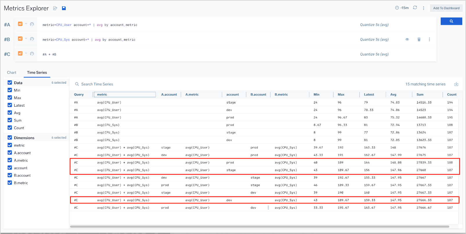
Given these example queries:

#A: metric=CPU_User account=* | avg by account,metric
#B: metric=CPU_Sys account=* | avg by account,metric
#C: #A + #B

Query #A returns three result sets:

metric=CPU_User, account=dev
metric=CPU_User, account=stage
metric=CPU_User, account=prod

Query #B returns three result sets:

metric=CPU_Sys, account=dev
metric=CPU_Sys, account=stage
metric=CPU_Sys, account=prod

Query #C returns 9 result sets:

(metric=CPU_User, account=dev) + (metric=CPU_Sys, account=dev)
(metric=CPU_User, account=dev) + (metric=CPU_Sys, account=stage)
(metric=CPU_User, account=dev) + (metric=CPU_Sys, account=prod)
(metric=CPU_User, account=stage) + (metric=CPU_Sys, account=dev)
(metric=CPU_User, account=stage) + (metric=CPU_Sys, account=stage)
(metric=CPU_User, account=stage) + (metric=CPU_Sys, account=prod)
(metric=CPU_User, account=prod) + (metric=CPU_Sys, account=dev)
(metric=CPU_User, account=prod) + (metric=CPU_Sys, account=stage)
(metric=CPU_User, account=prod) + (metric=CPU_Sys, account=prod)

Including along account in the query ensures that only result sets in which the value of the account field match should be used for computation. This narrows down the result set list to the result sets expected.

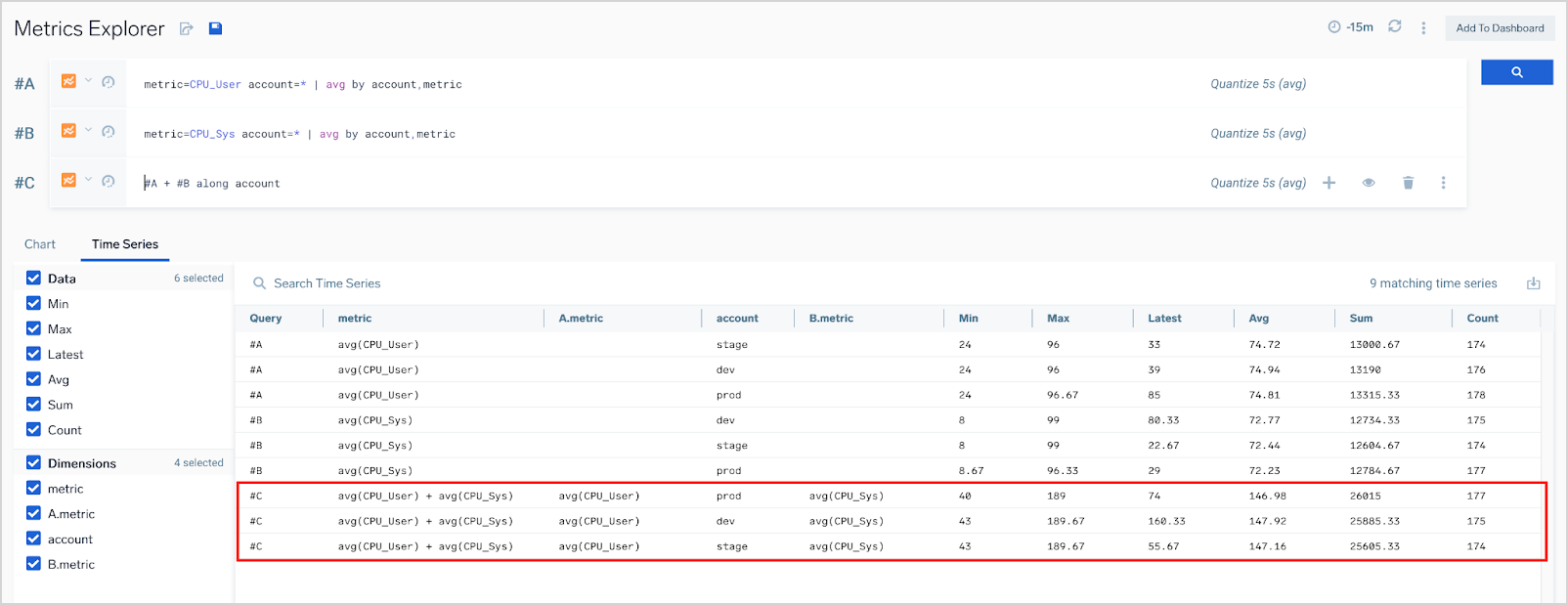
Queries with modified #C row:

#A: metric=CPU_User account=* | avg by account,metric
#B: metric=CPU_Sys account=* | avg by account,metric
#C: #A + #B along account

return same result sets for row #A and #B and only three results for row #C:

(metric=CPU_User, account=dev) + (metric=CPU_Sys, account=dev)
(metric=CPU_User, account=stage) + (metric=CPU_Sys, account=stage)
(metric=CPU_User, account=prod) + (metric=CPU_Sys, account=prod)

Quantization and joined queries

The results of a query with a join are calculated separately for every quantization bucket. This can produce unexpected results when time series with misaligned quantization buckets are joined.

For example, consider a joined query that compares the CPU_User metric from two different hosts.

#A: metric=CPU_User _source=”HostMetrics”
#B: metric=CPU_User _source=”JBM Host Metrics”
#C: #A+#B/2

Doing a quick comparison of metrics and average value over a short period can yield can surprising results, as the screenshot below illustrates.

note

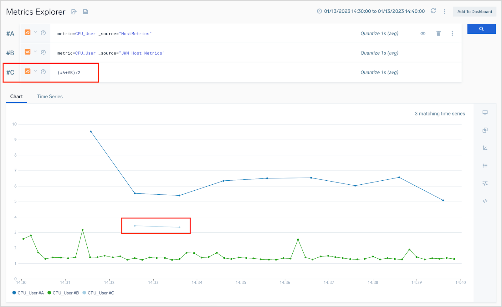
query #C computed the two values of the average value.

At the right end of each query row, you can see that that quantization period automatically optimized for the selected period is one second (quantize 1s (avg)). If the quantization bucket size (one second in this case) is less than the interval at which the metrics are reported, some of the buckets may not contain data points from both query #A and query #B. In our example, there were only two one-second buckets in which both hosts reported metrics.

To avoid this issue, you can specify a longer quantization bucket using the quantize operator. We recommend you explicitly set the quantization interval in queries that a joined query references. For example:

#A: metric=CPU_User _source=”HostMetrics” | quantize to 15s
#B: metric=CPU_User _source=”JBM Host Metrics” | quantize to 15s

along examples

Summation for a time series

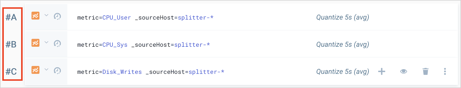
Queries #A and #B return the CPU_User and CPU_Sys metrics for time series whose _sourceHost dimension starts with the string cqsplitter-. Query #C performs a summation for the pairs of time series from #A and #B whose _sourceHost value matches.

#A: metric=CPU_User _sourceHost=cqsplitter-*
#B: metric=CPU_Sys _sourceHost=cqsplitter-*
#C: #A + #B along _sourceHost

Disk percent between available and free by device name

This query considers and returns a disk percentage metric available and free for devices with the same devName.  

#A: metric=DiskFree DevName=*
#B: metric=DiskUsed DevName=*
#C: (#B / (#A + #B)) * 100 as DiskUsedPercent along DevName

Sum and create a total metric

This query adds bytes_in to bytes_out for each node, and creates the metric bytes_total. Each time series in #A gets paired with an appropriate series from #B, the one that has the same cluster and node fields.

#A: metric=bytes_in node=* cluster=*
#B: metric=bytes_out node=* cluster=*
#C: #A + #B along cluster, node as bytes_total

Calculate percentages for nodes by cluster

This query calculates bytes_in as a percentage of bytes_total for each node. The expression allows referring to the same series more than once in the expression. In this example, #A appears twice in the expression.

#A: metric=bytes_in node=* cluster=*
#B: metric=bytes_out node=* cluster=*
#C: #A * 100 / (#A + #B) along cluster, node as bytes_in_pct_total

Queries with aggregate operator

When running a join queries with an aggregate operator, as a rule of thumb, include all the aggregation dimensions in the result query using along:

#A: metric=Net_InBytes | avg by _sourceHost
#B: metric=Net_OutBytes | avg by _sourceHost
#C: #B - #A along _sourceHost

Filtering by metadata

Filtering metrics using metadata can be useful when you have requirements like:

• "Show all metrics of CPU_LoadAvg for 1 minute, 5 minutes, and 15 minutes for top three servers according to the CPU_LoadAvg_1min", or
• "Show CPU utilization of the host with the highest memory consumption".

The query below simulates the effect of filtering on metadata from another row (#A) by using a metric join that includes only data for metrics available in results from that other row. This example effectively filters results from row #B to leave only those with the _sourceHost value returned query #A:

#B + 0 * #A along _sourceHost

The easiest way to analyze this query is going from the end backwards. In this query, for each quantization bucket we get data for all _sourceHost dimensions from results of row #A, then we multiply it by 0 so we get value of 0, then we add 0 to the results of row #B for same _sourceHost and quantization bucket. At the end, the result is provided only for quantization buckets where values are available for both referenced result sets and for _sourceHost dimensions which are returned by both #A and #B. This has some side effects:

• There are no results for metric dimensions which are not available in any of the rows.
• There are no results if data points fall into different quantization buckets.

An advanced version of this query shows all metrics of CPU_LoadAvg for 1 minute, 5 minutes, and 15 minutes for top three servers according to the CPU_LoadAvg_1min (in the result sets returned by rows #A, #D and #E):

#A: _sourceHost=nite-metricsstore-* CPU_LoadAvg_1min | topk(3,avg)
#B: _sourceHost=nite-metricsstore-* CPU_LoadAvg_5min
#C: _sourceHost=nite-metricsstore-* CPU_LoadAvg_15min
#D: (#B + 0 * #A) along _sourceHost
#E: (#C + 0 * #A) along _sourceHost

We use results from row #A here, both for comparison on a chart and as a filter in rows #D and #E.

Troubleshooting tips

• Misaligned quants. If you see fewer results than expected (or no results at all), most likely you should most increase the size of the quantization bucket. For more information, see Quantization and joined queries.
• Missing along. If you see more results than expected (or unexpectedly exceed the maximum output cardinality), you probably forgot to add along to your query. For more information, see Understanding along.